Excel is the go to problem solving platform in current day and age. With the advent of artificial intelligence, where everything seems to fall in singularity and revolve around AI prompts, Excel is still leading and pushing the boundaries with latest and practical integrations including Excel Copilot.
In this tutorial:
Understanding the legacy, importance and how its evolving, one cannot ignore but learn Excel.
Understanding Excel Interface
Excel’s first sight might overwhelm the first time you open it with unusual number of rectangles offering no help or clue on what it does and how. But don’t worry, let’s understand each part one by one starting with the labeled diagram of the user interface.
Just go through the following, no need to memorize it, to understand what each element is about.
Pro Tip: While working inside Excel, you can hover above particular element to know the name and purpose of it.
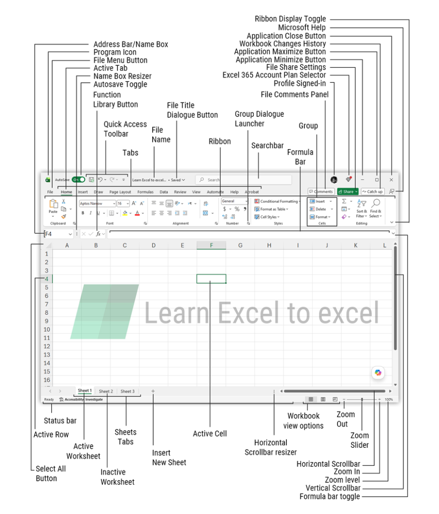
Following table describes what each item is and very briefly its function:
| Item/Feature | Description |
|---|---|
| Address Bar/Name Box | Shows the address of active cell or the name incase of defined data range. |
| Program Icon | Excel Logo. On left clicking application menu will appear with options to minimize, maximize, restore, close options. |
| File Menu Button | Opens a page with options start new workbook, open a previously saved book, to save file, print options, access to document information, excel settings and account options. |
| Active Tab | The tab which is currently in front and the contents under this tab are displayed and other tabs are hidden. By default home tab is an active tab. But clicking other tabs name will make them active which gives access to different options. The contents of active tab are shown as Ribbon |
| Name Box Resizer | |
| Autosave Toggle | |
| Function Library Button | Pressing this button opens up dialogue box where you can select different formulas available in excel. Frequently used formulas are listed but user can also search for formula easily |
| Quick Access Toolbar | As the name suggests holds icons to functions that are often used and this bar make them readily available to be accessed quickly. It can be customized to suit users’ needs. |
| Tabs | These are the tabs in which different functions are organized with relevant functions for easy access. |
| File Name | This is the name of excel file that user has input while saving it. By default excel files are named as Book 1, Book 2 etc |
| File Title Dialogue Button | |
| Ribbon | |
| Group Dialogue Launcher | |
| Searchbar | |
| Formula Bar | If user has inserted a formula in a cell then it will be shown in this bar or field. |
| Group | A subdivision inside ribbon where icons of relevant features having similar purpose are placed together for easy access. |
| File Comments Panel | |
| Profile Signed-in | |
| Excel 365 Account Plan | |
| File Share Settings | |
| Application Minimize Button | This minimizes the excel window/application to windows taskbar |
| Application Maximize Button | This button will maximize the excel window/application to whole screen. |
| Workbook Changes History | |
| Application Close Button | This will shut down the excel program including all the opened workbooks and windows |
| Microsoft Help | |
| Ribbon Display Toggle | This minimizes the excel ribbon upwards increasing the workspace for user. Shortcut to minimize excel ribbon Ctrl+F1 does the exact same function |
| Status Bar | |
| Active Row | The numbers at the left of worksheet are row numbers. The active row is highlighted with changed colour which is golden that helps easy identification |
| Select All Button | Clicking this button will select all the cells in the worksheet. |
| Active Worksheet | The worksheet which is on screen at the moment. The active one appears brighter than others. |
| Inactive Worksheet | |
| Sheets Tabs | Group of worksheet tabs that a workbook holds. |
| Insert New Worksheet | Clicking this button will add one more worksheet to workbook. |
| Active Cell | Excel’s worksheets are divided into cells. Each cell is an entity that can hold its own information or from other sources. The cell that is active has black border or enclosed in a box with a small extension at the bottom right corner called handler. |
| Horizontal Scrollbar Resizer | Dragging it will expand or reduce the size of horizontal scroll bar. |
| Workbook View Options | Three viewing options from which user can select and switch to another view on the go by clicking each option. Options are Normal, Page layout and Page break preview. |
| Zoom Out | This decreases the size of the worksheet and its contents |
| Zoom Slider | Dragging this handle will zoom in or out the worksheet |
| Horizontal Scrollbar | This bar helps scroll the worksheet right or left. |
| Zoom In | This increases the size of worksheet and its contents |
| Zoom Level | In percentage this provides information how big the data is being displayed in relation to its real size. 100% is default value |
| Vertical Scrollbar | |
| Formula Bar Toggle | This expands and collapses the formula bar that helps in reading long formula |
Data Entry: Making your First Workbook
After learning the basic interface we can proceed with entering data in the worksheet.
Inputting the data, formally called data entry, is quite easy. Simply select any cell and start typing. Data can be text, numbers of mix of text and numbers. Pressing the Enter key on the keyboard completes the data entry in one cell and automatically moves to the next cell.
In addition to manual data entry, we can also copy and paste the data among other ways to get the data in Excel worksheet.
Formatting Data in Excel
Once data entry completes, we can work on data appearance formally called data formatting. Formatting data helps understand the data better by differentiating each element of the data.
Excel offers numerous options under the Home tab categorized in different groups like Font, Alignment, Styles etc.
To apply or change a format like font size or style, we can simply select the cell or cells and click the appropriate button in the top ribbon.
Excel also offers dedicated keyboard shortcuts for certain tasks or tools. This saves users time and effort to manually find and click the button in the ribbon. For example, to change the font style in a cell simply hit CTRL+B. [Excel Shortcuts Article/Cheatsheet]
More about alignment which will complete text related formatting
Continue with number related formatting and how Excel offers several options for this.
Move on to adding and deleting rows from the data. And then to formatting the tables manually then with built-in styles and then table.
Lastly expand on Conditional Formatting.
Excel Functions and Formula
With data available and presentable in the worksheet, its time to learn the very reason Excel exists in the first place i.e. Functions and Formulas.
Most of the time the terms functions and formula are used interchangeably but difference is there:
- Excel functions are pre-built programs to perform a certain tasks.
- Excel formula is a set of instructions by the user that may contain a function or multiple functions to perform a certain task.
In other words, a formula is user-defined program that may or may not contain pre-built programs i.e. functions.
Every formula starts with an equal sign “=”. Basic formula involve arithmetical calculations like sum, multiply, divide etc.
Write up about how formula is constructed in simple words involving cell addresses.
SUM
Consider the following data that contain sales data and we want to sum the sales for both years for each product. For the first product, sales are in cell B2 and C2 for each year.
To sum the values in both cells we need to put the following formula in cell D2:
=B2+C2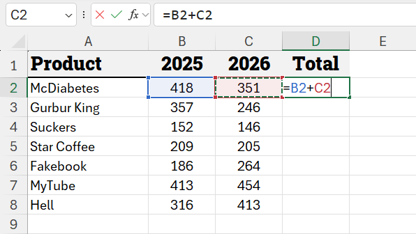
Similarly, we can refer to respective cells in each row to find the total sales for other products by typing the formula.
Alternative to our formula, Excel has a built-in function named SUM. Instead of selecting each cell separately and joining each cell with a plus sign, we can use SUM function and select all the cells to get the total sum. The formula to get the first product is:
=SUM(B2:C2)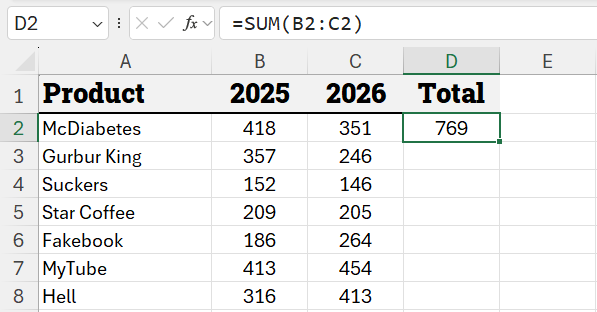
Instead of manually writing this formula for each row, simply type the formula in the first row and double click the fill handle and Excel will automatically apply the same formula for the entire data.
Excel also has a dedicated shortcut to insert sum function for similar data sets. Simply select the numbers you like to add including the column or rows where you want to insert totals and hit ALT+= on the keyboard and Excel will instantly calculate totals for each row by auto inserting SUM function in each row.
After learning SUM function, following are some of the basic Excel functions to learn next:
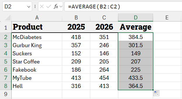
AVERAGE
Calculates the average of the numbers in the specified range.
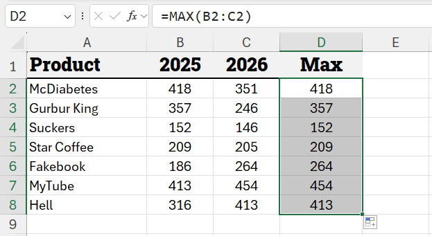
MAX
Gets the largest value in the selected data range
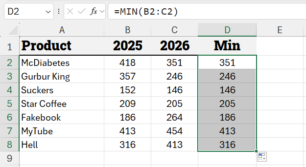
MIN
Finds the smallest value in the data.
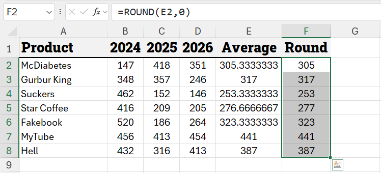
ROUND
Rounds the number to specific number of digits. Additional related functions are ROUNDUP and ROUNDDOWN.
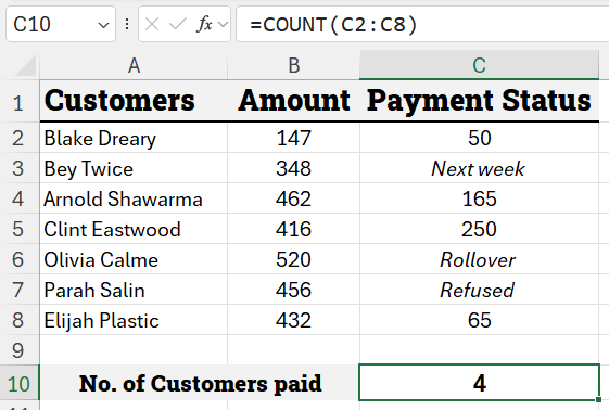
COUNT
Counts the number of cells within the selected range that contain numbers.
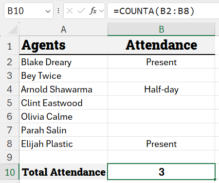
COUNTA
Counts the number of cells that are not empty.
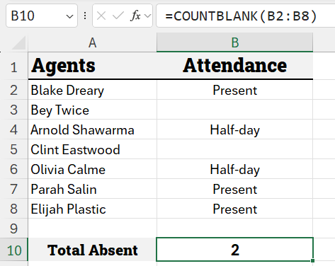
COUNTBLANK
Counts the number of cells that are empty.
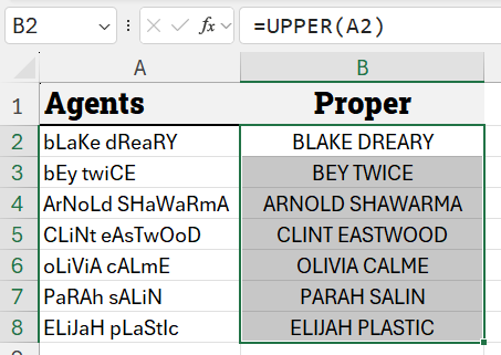
UPPER
Converts the text to upper case.
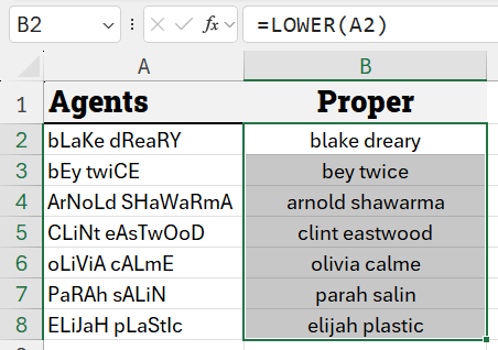
LOWER
converts the text to lower case
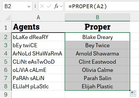
PROPER
Processes the text to proper case.
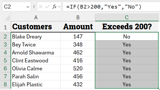
IF
Check if a condition is true or false and returns specified result accordingly.
Excel Charts: Giving your data eyes
After learning basics of data entry, data formatting and data processing with formulas, lets learn how to visualize data using Excel charts.
Excel offers charts of different shapes and users can decide which one to use based on visual preference and purpose.
To plot the following data of three years, select the data by having active cell within the data and hit CTRL+A. Go to Insert tab > click Recommended Charts button > Press OK on the dialogue box and Excel will insert the chart as below:
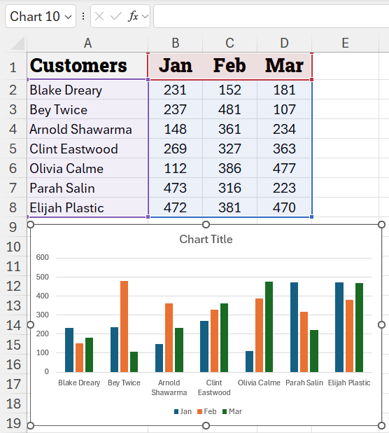
Excel charts are very customizable as one can make changes to each and every element of the charts or choose between different types of charts e.g. bar charts, column charts, pie charts, hierarchical charts etc.
In addition to charts, Excel also offers in-cell charts called Sparklines.
Excel Sparklines
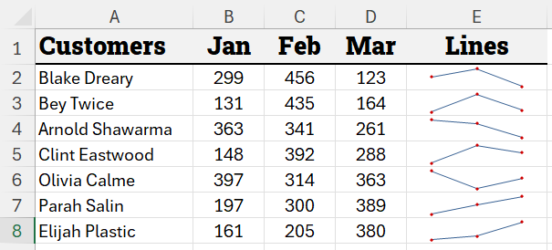
Sparklines are Excel’s compact in-cell charts for users understanding of the data with a quick glance.
As of now Excel Sparklines has three variations named; Line, column, Win/Loss. Becomes a lot easier to spot the trends with this tool as data is along the same row and numbers alone hardly help in most of the cases.
To insert the sparklines go to insert tab > under sparkline group click line > select the range > press OK. Drag the fill handle down to insert sparklines for rest of the rows.
Custom In-cell Charts using Formula
Sparklines are quite limited when it comes to customization. To achieve the similar results with more flexibility, users can learn the in-cell charts technique using formula with specific fonts.
Excel Data Tools
Excel offer multiple built-in tools for data processing and manipulation. These tools cater the tasks users often needs to carry out and they can do it with a dedicated dialogue box, user interface or simply dragging and dropping the elements.
Following are some of the notable tools every Excel beginner must learn and practice to become proficient in Excel.
Text to Column
Text to column is a dedicated tool to split text data in a single column to multiple columns based on specific delimiter or delimiters. Where delimiter is simply a character, symbol or else used to determine pieces of data that needs to go in separate column.
Excel’s Text to column is especially useful in CSV files where data is formatted in a way that values or parts of data are separated by commas.
A delimiter can be a space, comma, semi-colon, period, slash, pipe symbol etc.
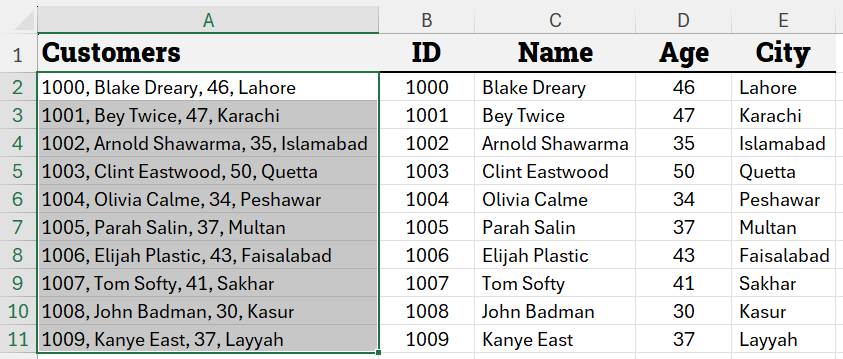
Following is a comma separated data that we want to split in relevant columns:
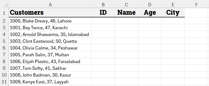
Select the data and go to Data tab > under Data Tools click Text to Columns button:
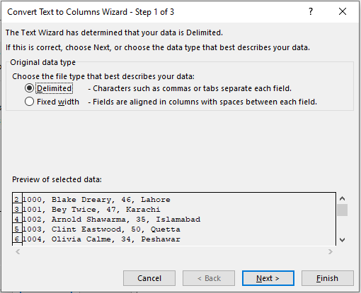
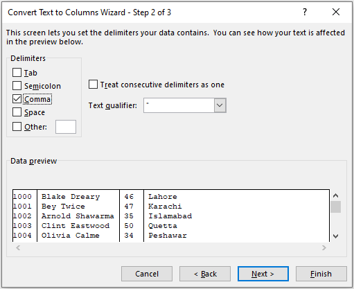
In the dialogue box, click Next button, select the appropriate delimiter which in our case is comma. Preview of how the data will split is shown within the dialogue box. Click Next:
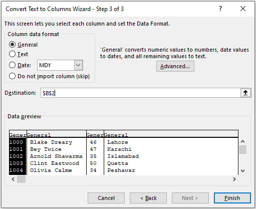
In the next window, select the cell where you want the output, in our case its B2, click Finish:
Here is the data split into multiple columns:
Remove Duplicates
Remove duplicates tool does exactly as the name suggests. A simple yet effective tool.
Have a look at the following data infested with duplicates:
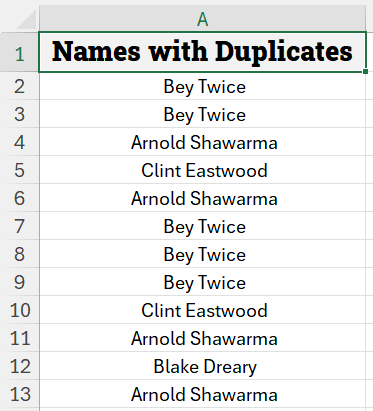
To remove the duplicates, select the data > go to Data tab > under Data Tools click Remove Duplicates tool, the following dialogue box appears:
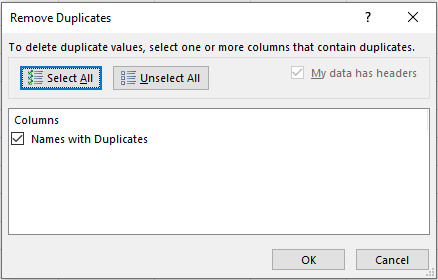
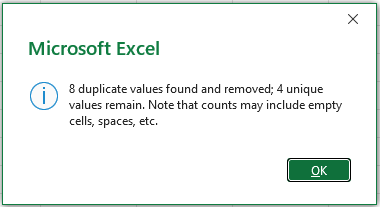
Click OK and Excel will remove the duplicates and display the information as following:
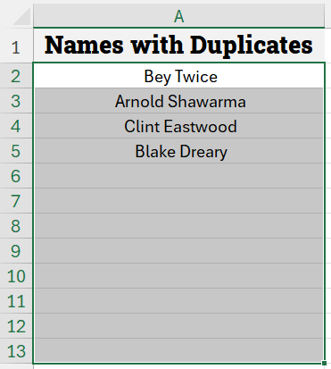
Following are the results with duplicates removed:
Sorting Data in Excel
Excel Sort Tool
Excel offers Sort tool to sort data in ascending or descending order. Moreover, we can sort multiple columns at once that is technically called multi-level sort.
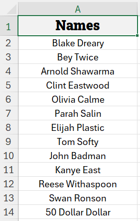
Consider the following unordered data:
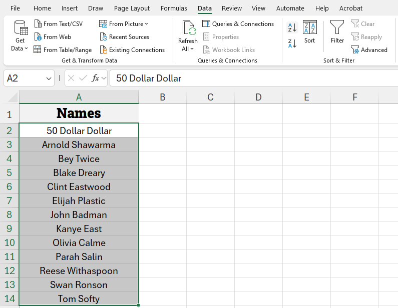
To sort data in ascending order, simply select the unordered data excluding the heading > go to Data tab > click Sort A to Z button and Excel will sort the data in ascending order:
Similarly, to sort the data in descending order, select the data again and click the Sort Z to A button:
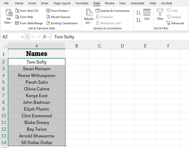
Excel can sort even multiple columnar data sequentially.
For example, if we want to sort one column in ascending order and the next one in descending order, Excel sort tool can do so let you do it with a user-interface.
Here is one example of unsorted data with multiple columns:
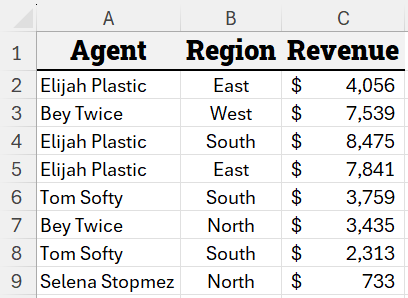
To sort Agent column in descending order and Region in ascending order, select the entire data > go to Data tab > under Sort & Filter group click Sort button. Following dialogue box will appear:
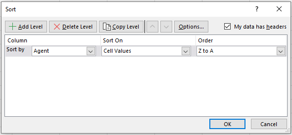
For the Agent column, the order is already descending, click Add level bottom at the top left column and select Region from the drop down and select A to Z in the order drop down and click OK button:
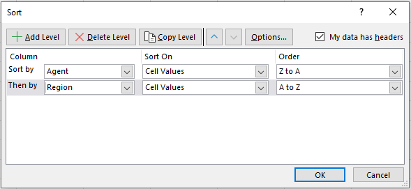
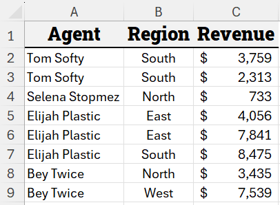
And here is the data sorted:
Excel SORT Function
Excel also offers SORT function in addition to sort tool. Excel SORT function is more flexible and practical than the tool version as it dynamically outputs data anywhere user wants instead of permanently rearranging the data in its place.
SORT Function vs Sort Tool
| Feature | SORT Function | Sort Tool |
|---|---|---|
| Type | Formula | Tool |
| How to access? | Within cell just like any other function | From Ribbon under Data tab |
| How it works? | Spills the results into a new range with original data intact | Permanently rearranges the original data |
| Affects original data? | No | Yes |
| Best for? | Dynamic reports, dashboards, formulas | One time data organization |
| Static or Dynamic? | Dynamic; output will update as and when the original data changes | Static; user have to redo every time original data changes |
| Formula Support? | Yes, easily integrates with other functions to create a formula | No way to integrate its working or output within formula |
| Multi-level Sorting | Yes, requires the knowledge of array constants | Yes, use the options in the dialogue box |
To learn more on how to sort data using formula in Excel check this guide.
Data Validation Tool
Data validation tool is one of the most important features every Excel user must learn thoroughly.
Its job, as the name suggests, is to validate the data i.e. it stops the wrong data to enter the file right at the time of entry. This tool offers multiple options to restrict user to provide only the correct data to ensure data accuracy.
To apply data validation rules, simply select the cell or range of cells and go to Data tab > under Data Tools group click Data Validation button. This will open a Data Validation dialogue box.
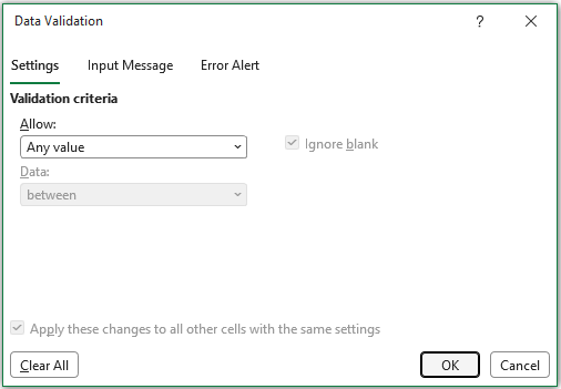
The dialogue box contain three tabs:
- Settings
- Input Message
- Error Alert
The Settings tab house the validation criteria and user has several ready made validation rules to choose from with additional options for each to fine tune further.
Input Message tab lets users customize the input message box that appears if cell or cells with validation rules are selected. Message box is mainly provided to let users know what type of data is expected. If no input message is defined, no message box will appear for such validation rules.
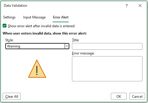
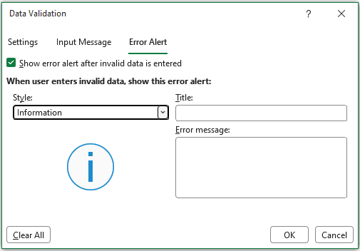
Error Alert tab contains the customizable options regarding message box that appears if validation rules are not followed and how to handle error situations. It offers three options:
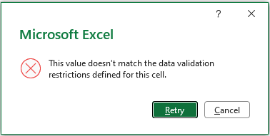
Stop: On detecting invalid input, stops the user from entering such data with the specified message.
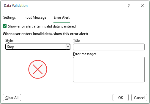
User is offered either to retry entering the correct data or cancel the input attempt altogether.
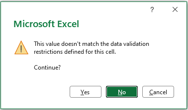
Warning: Invalid input is accepted but a warning message box is displayed notifying the user that data is incorrect.
User is offered three options; Yes to accept the invalid data, No to retry data entry or Cancel to delete the invalid entry.
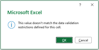
Information: Invalid input is accepted but a message box is shown to the user notifying that input is not correct.
User has two options; OK to accept the data entered as is or Cancel to delete the input.
The tool offers several ready made validation criteria like:
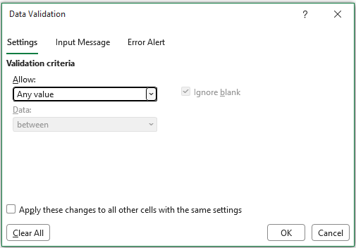
Any value: by default this is selected for every cell and user can enter data with no restrictions.
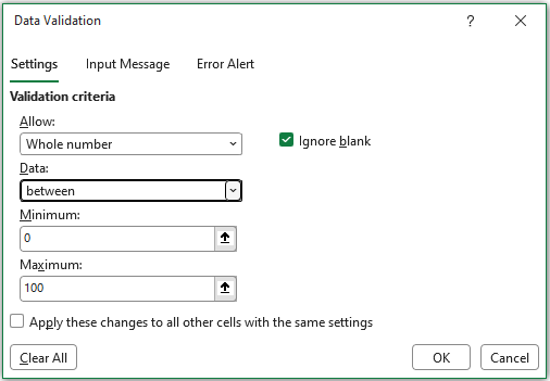
Whole number: user can enter only whole numbers with additional criteria to be set. For example, limit the allowed input between minimum and maximum.
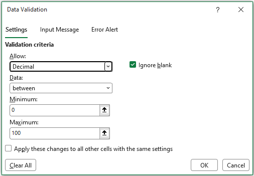
Decimal: user need to input just numbers that can either be integers or decimal numbers. Basically a step up from whole number criteria that accepts just whole number, this criteria accepts decimal numbers as well.
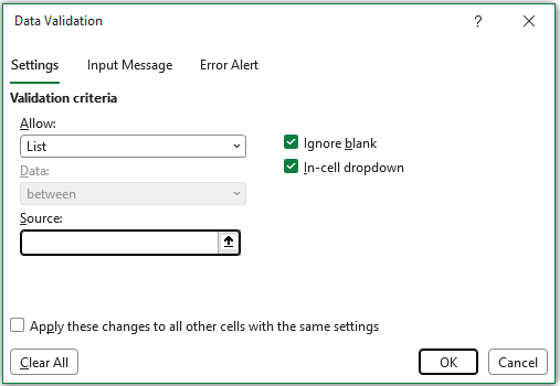
List: can select only predefined choices from the list that are either provided manually or from a specific range or generated through a formula. This is shown as a drop-down menu that allows user to make the selection easily. If drop-down option is unchecked, dropdown menu is not available and user can enter only such data that is included in the list.
Date: with this criteria selected, only dates can be entered. And just like we saw in Whole number and Decimal criteria, we have additional options to restrict the input.
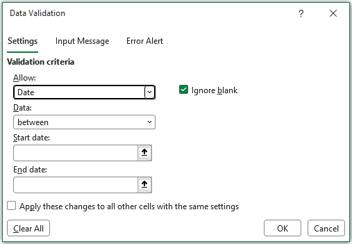
Time: such cells can take only time value
Text length: restricts the user to input data of specific character length
Custom: accepts such input that fulfills the formula based criteria. This option unleashes the potential of validation rules as you can define complex conditions using formula beyond limited whole number and decimal limited criteria.
Pivot Tables
Pivot tables is an analysis tool that summarizes the data by reorganizing or “pivoting” the data by simply dragging and dropping the column headers in the dedicated user interface without the need of any formulas.
For instance, if we want total sales for all the products, pivot tables allows us to make this report in seconds by identifying the products to get a unique list and then sum the sales for each product that is presented in the form of a table.
Have a look at the following data, and we want total sales by each Agent:
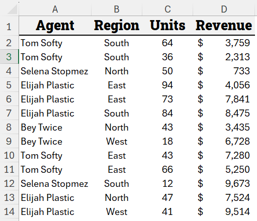
To find the totals by each sales person, we can use Excel pivot tables. Simply have an active cell within the data > go to Insert tab > under Tables group click Pivot Table > following dialogue box opens:
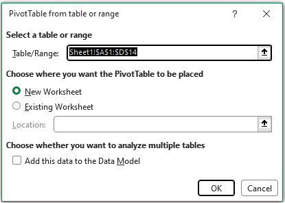
In this we can choose to insert the pivot table on a new worksheet or on the existing worksheet. Click existing worksheet and select the cell of your choice e.g. F1 and click OK. This will invoke Pivot table user interface as a sidebar and pivot table report within the worksheet:
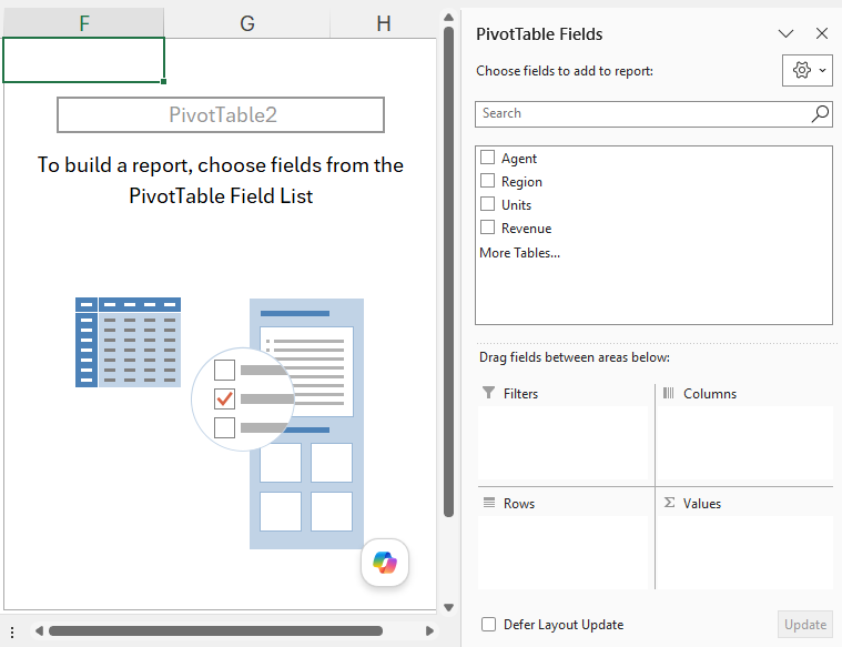
As we want totals by sales agents, press and hold left mouse button on the agent field and drag it into the rows box. Afterwards, drag the revenue field in the values box. Here are the results:
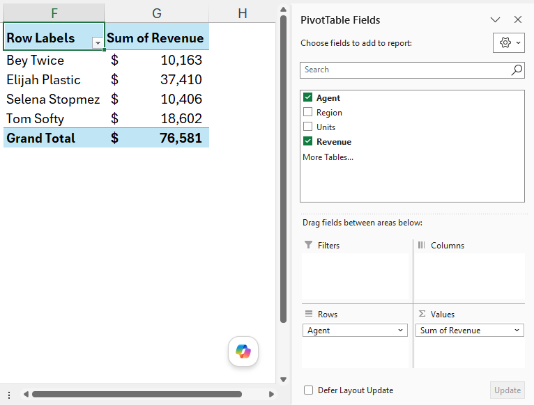
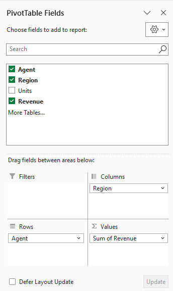
Similarly, to know the sales total of each sales agent by the region as well, simply drag the region field in the columns box as following:
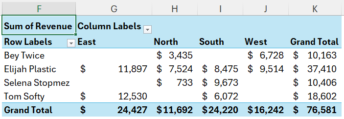
And we get the total sales for each sales agent by the region as following:
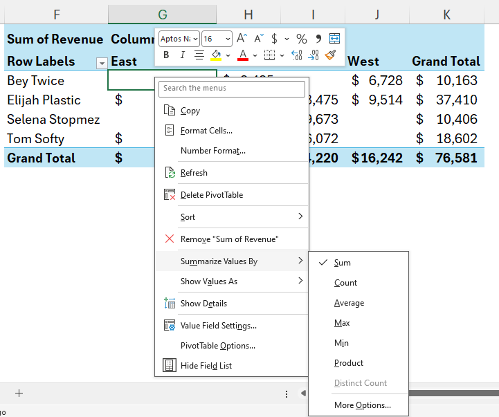
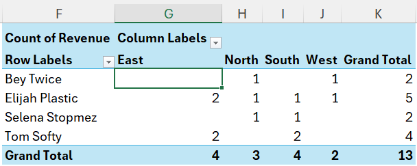
Similarly, to know the total number of sales instead of amount by region made by each sales agent, simply right click on any cell within the pivot table report > hover on “Summarize values by” > click Count:
And this will update the report with the number of sales instead of amount of sales:
Power Query
Power Query is a data preparation and transformation tool in Excel that eliminates the need of complex formulas and coding with a user friendly interface. This tool allows the users to carry out complex ETL tasks i.e. extract, transform and load at the click of a button without altering the original data.
Power Query lets users to get the data from multiple sources dynamically inside Excel. One can import data from text or CSV files, web, PDF files and even images. Once data is imported, user can link the data together and design the processing model that includes repetitive tasks within Power Query environment and load the finished data as one unit in Excel worksheet.
Get data from file
Power Query let users import the data from multiple sources including text files, CSV files, PDF files, other Excel workbooks etc.
In the following, data is stored in text file that we like to import in Excel:
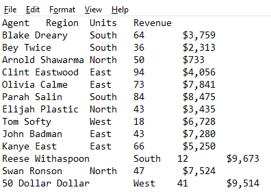
Go to Data tab > under Get & Transform Data group click Get Data > go to From file > click From Text/CSV
A browse window will open. Navigate to location where the file is stored open it. This will invoke import box within Excel:
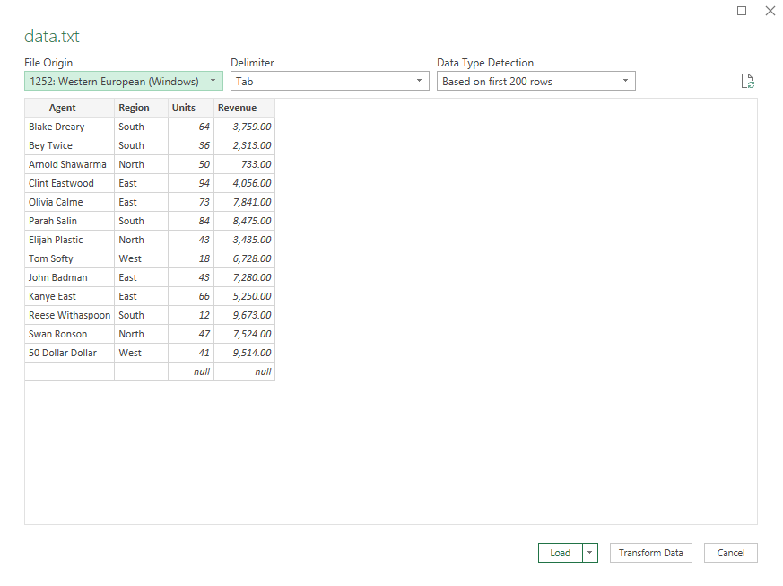
Click the dropdown by the Load button and click “Load to…” and another box will popup letting you select where to paste the data:
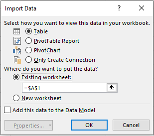
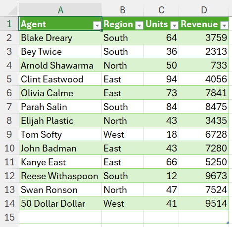
After selecting the appropriate location, press OK and Excel will import the data:
Remove Duplicates using Power Query
Power Query can help you remove duplicates easily with a click of a button.
Consider the following data with duplicates and we like to remove them using Power Query:
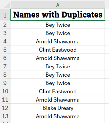
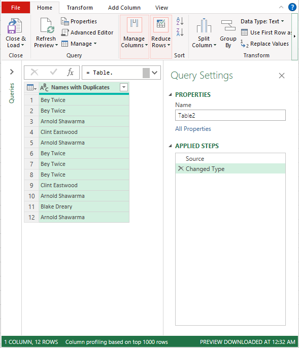
Select the entire data including the headers, go to Data tab > under Get and Transform Data click From Table/Range. Click OK on the pop-up box. This will convert the range in table Table and opens the Power Query editor:
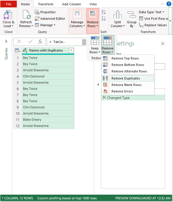
Go to Reduce rows > click Remove rows > click Remove Duplicates:
This will immediate remove duplicates from the data rendering the clean data to be inserted in the worksheet:
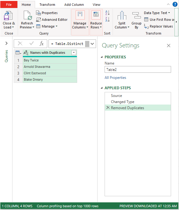
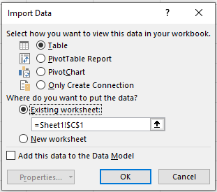
Click Close & Load button and click Close and Load to… option and from the window select existing worksheet and then select the cell where you want to insert the processed data and click OK:
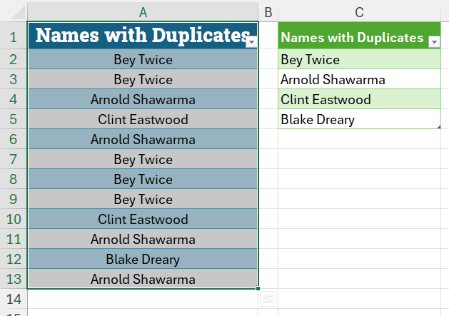
Following is the result:
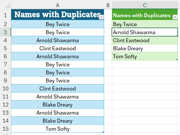
Benefit of this method is that if new data is inserted in the original data table, we simply need to refresh the query and it will process the data automatically without the worry of duplicates:
Get data from image
Excel Power Query now lets users to extract and import data even from image files.
Here is one example of an image with data we like to import:
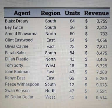
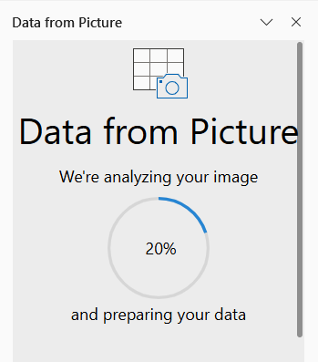
Go to Data Tab > under Data & Transform Data group click “From Picture” > click Picture from File. From the browse box, navigate to location of the image and open it. This will start data extraction engine in the sidebar:
Once the analysis completes, Excel gives the data extracted that requires user’s review before its inserted in the worksheet:
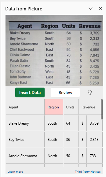
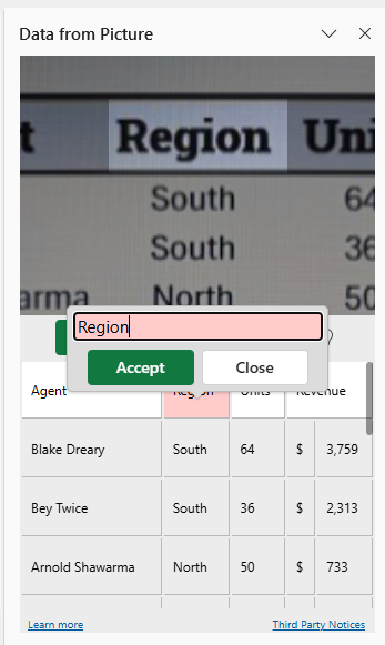
The content marked or highlighted requires user’s attention or probable edit. One can edit any data by simply click and inserting the correct data in the dialogue box:
Once all the data has been reviewed and corrected, click insert data button and Excel will insert the data where the active cell is within the worksheet:
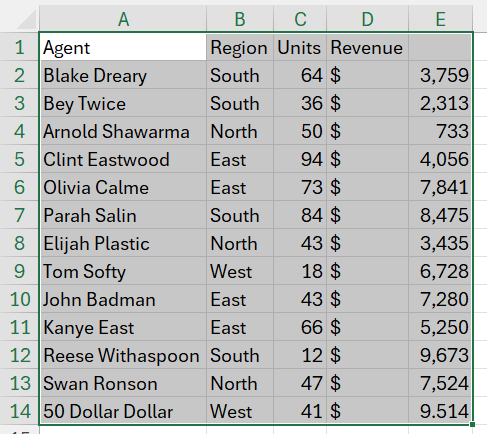
User might still have to clean up, as the feature itself is limited to extracting data and doesn’t offer much support in cleaning data. As in the above picture, currency sign is taken as a separate data value. Following is the corrected data with unwanted column removed, heading shifted to correct column and numbers formatted with currency sign:
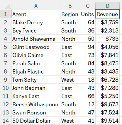
Combine data from multiple worksheets or files
To combine data from multiple worksheets within the same workbook, first convert each range to table by selecting and pressing CTRL+T.
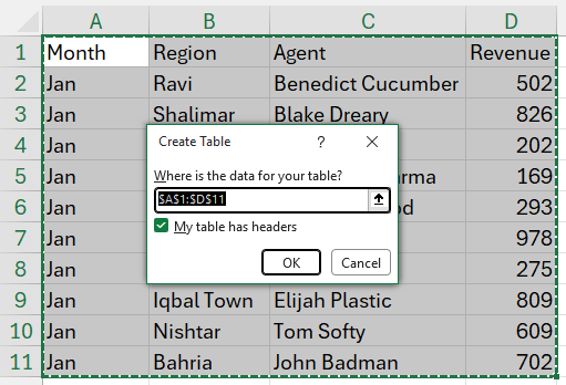
Once all the data ranges are converted, go to Data tab > click Get Data > hover over From other Sources > click Blank Query. This will open Power Query Editor interface. In the formula bar input the following and press Enter:
=Excel.CurrentWorkbook()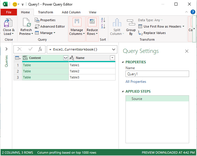
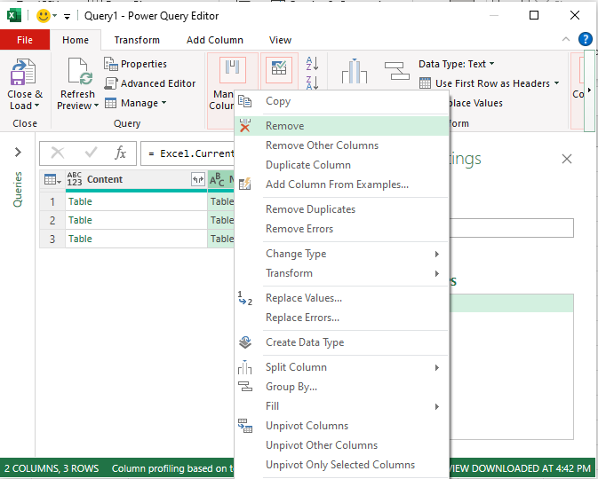
Power Query will fetch the tables and data. Remove the name column by right-clicking on the header and clicking Remove:
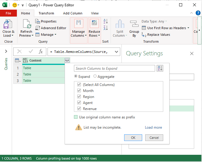
With irrelevant column removed, click the expand button that is on the right corner of the header and uncheck “Use original column name as prefix and click OK:
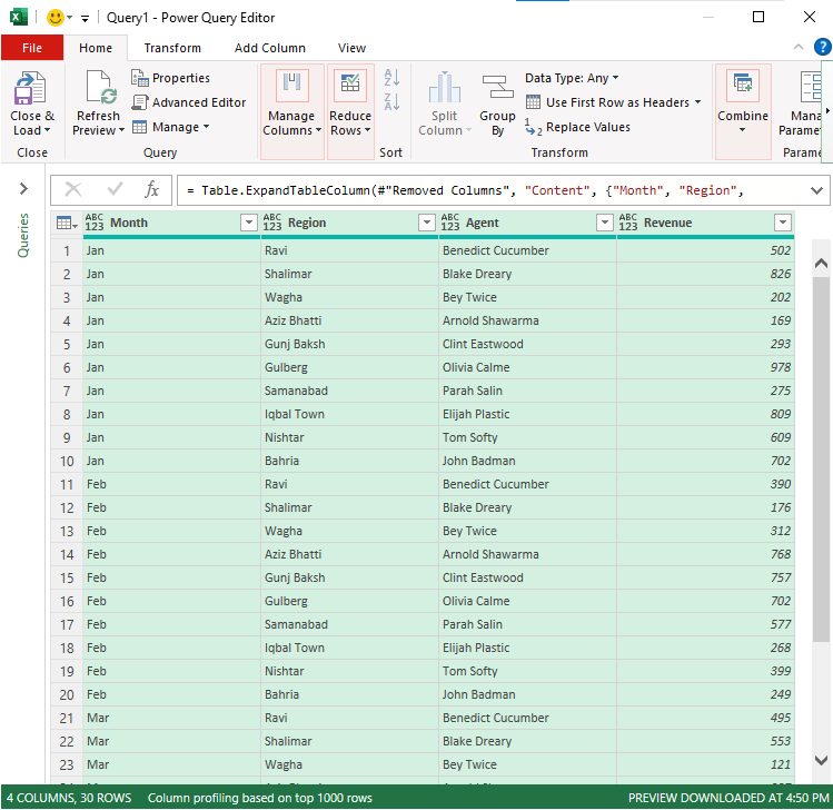
This will load the data from all the tables combined in one table:
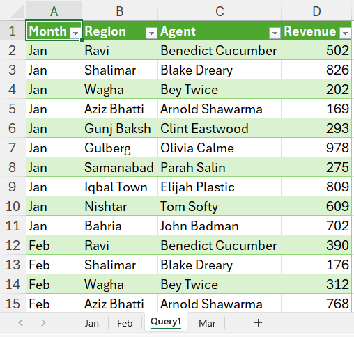
Click Close and Load button and the combined data will be inserted in the new worksheet with all the ranges combined:
Unpivot data using Power Query
Unpivoting the data is one of the necessary steps to normalize the data so that it can be worked upon easily.
Unpivoting the data is basically restructuring of data in a way that converts wider data into a columnar or vertical data.
Following illustration depicts the “wider” data range where sales of each year is put in individual columns:
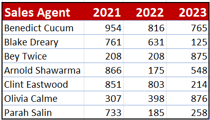
Instead of having revenue for each year spread across multiple columns, we should have a year column with year number and a revenue column containing corresponding amount. This converts the data into a taller, vertical data instead of wider data range. Hence the name “unpivot”.
To unpivot the data using Power Query, select the data range and press CTRL+T shortcut to convert the simple range into table range:
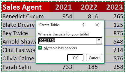
Once converted, go to Data tab > click from Table/Range. This will load the data in Power Query editor:
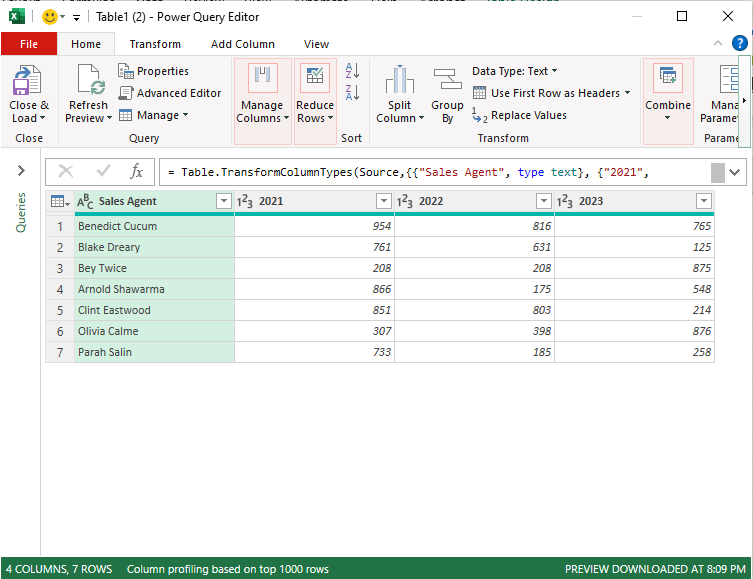
Select all the columns containing revenue by clicking the header of the first column, press and hold down Shift key and click on the header of the last column to select all the columns:
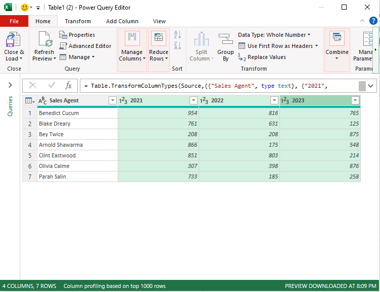
Go Transform tab > click Unpivot columns button and Power Query will instantly unpivot all the columns:
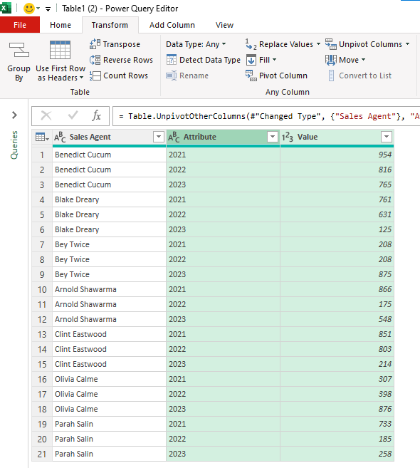
Rename the columns as Year and Revenue by double clicking respective header. Once done click Close and Load button under Home tab to insert the unpivot column in the new worksheet:
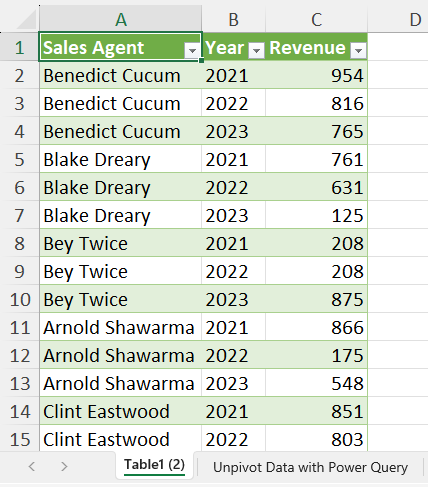
Extract data from mixed data
To extract data i.e. text data and number data into separate columns from the mixed data, Power Query can help to get this done easily.
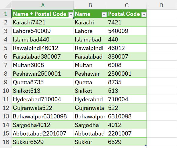
Here is one illustration with mixed data and we want to separate text data and numbers in separate columns using M code:
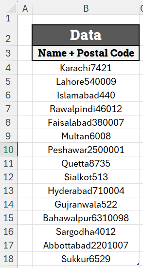
Select the range and convert it into table range. Once converted, go to Data tab > click From Table/Range button. It will open Power Query editor with mixed data imported:
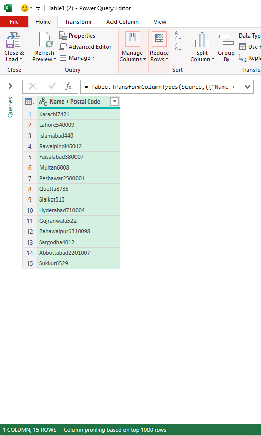
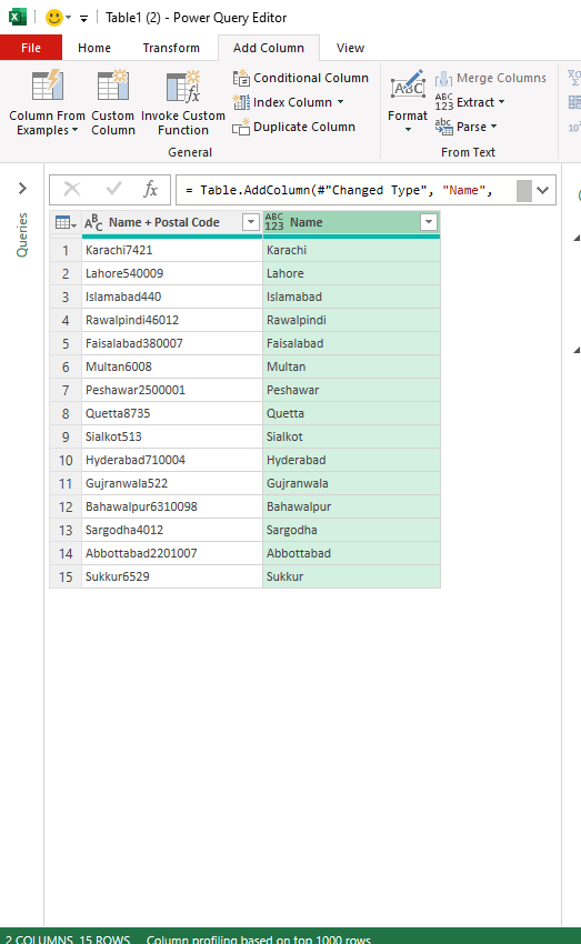
Go to Add Column tab > click Custom Column. In the window, enter Name as the new column name and put the following in the custom column formula box and Press OK button:
=Text.Select([#"Name + Postal Code"],{"A".."Z","a".."z"})This will extract the text part in the mixed data:
To extract number part, go to Add column tab again and click Custom column button. In the window, give column name as “Postal Code” and put the following code in the formula box:
=Text.Select([#"Name + Postal Code"],{"0".."9"})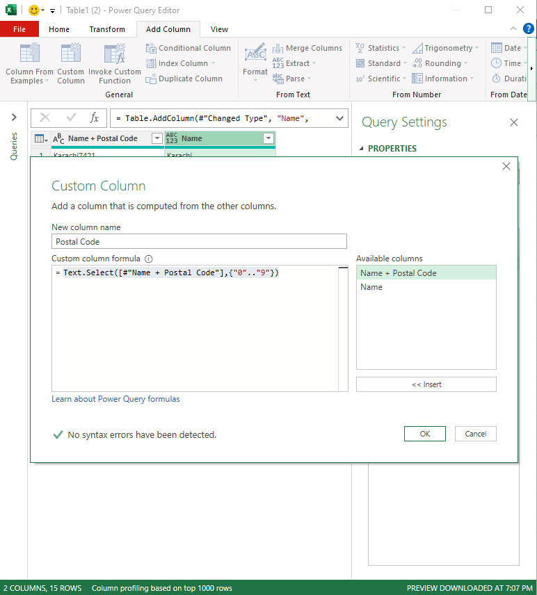
Press OK and new column will be inserted with postal codes extracted from the mixed data column:
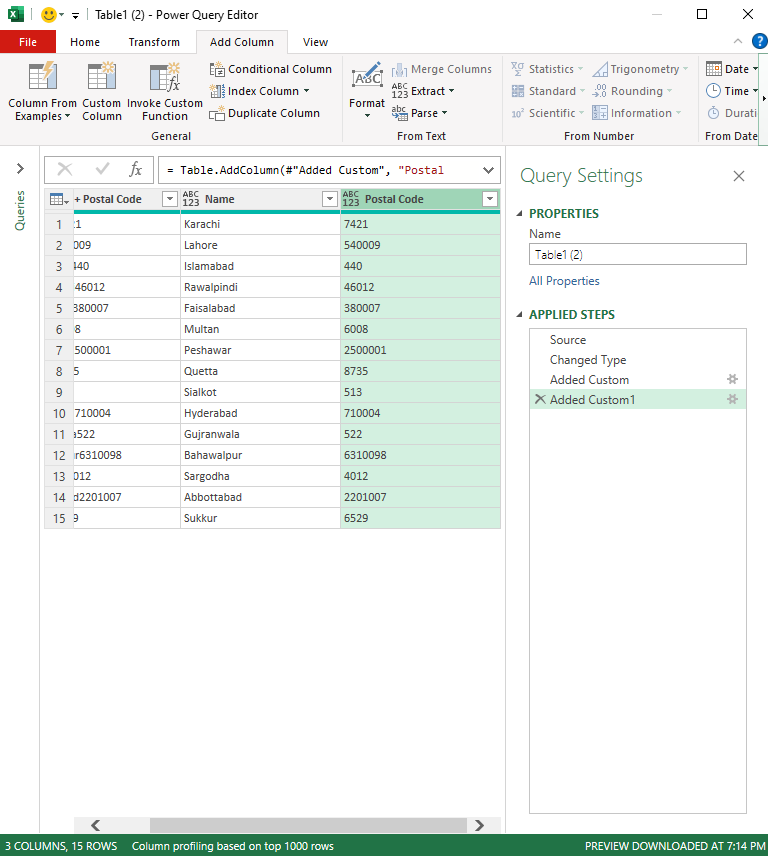
Go to Home tab and click Close & Load button. This will insert the processed data in the new worksheet: