Excel FILTER function allows us to delete blank rows from the data dynamically using a formula in Excel.
In this tutorial:
Before FILTER, Excel users were limited to removing empty rows either manually or using static tools like Find tool, Filter tool or Go to Special tool to identify, select and delete blank rows. Though, these tools still work, their use is cumbersome, error-prone and above all user needs to use them every time data has additional blank rows.
FILTER formula to remove blanks
FILTER allows us to extract data based on criteria. Using this facility, we can design a criteria rule that identifies blank cells or rows and remove them from the filtered results.
Delete Blank cells from a single column
In the following example, we have a column of data with blank cells. To get a clean data without empty cells, we can use following FILTER formula:
=FILTER(A3:A14,A3:A14<>"")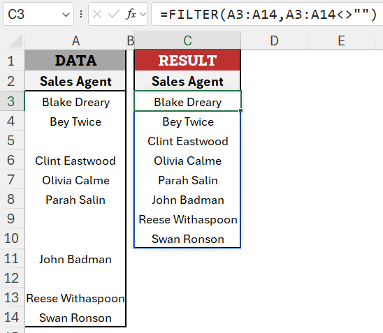
Lets take a step back and understand how this formula works.
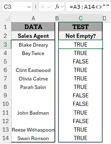
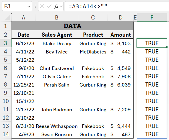
Taking the same data with blanks, lets test the whole range A3:A14 for empty cells. For this purpose use following formula:
=A3:A14<>""This criteria or formula tests if a cell is empty. <>”” means not equal to empty.
So the non-empty cells return TRUE and the empty ones returns FALSE. As a result we have a column with TRUE and FALSE values.
Using the same criteria in FILTER function under include argument we can filter out blank rows. We can even see the same Boolean output of this test within formula by selecting the criteria part and pressing F9 key on the keyboard:
=FILTER(A3:A14,{TRUE;TRUE;FALSE;TRUE;TRUE;TRUE;FALSE;FALSE;TRUE;FALSE;TRUE;TRUE})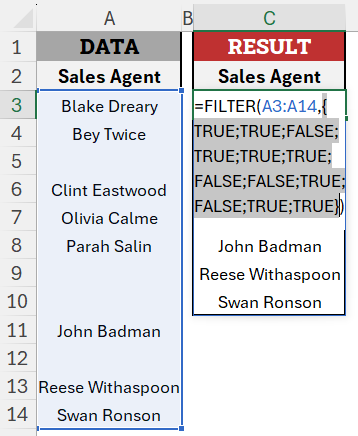
The cells containing data returned TRUE as one can see for the first two cells of the data. The third one cells is empty therefore returning FALSE in the array argument.
FILTER function outputs values that fulfill criteria i.e. TRUE results only and skipping FALSE. This is how blank cells were eliminated from the formula result.
FILTER formula to Remove Blank Rows
To automatically delete blanks rows from the data with multiple columns, we can use the same technique we learnt above.
Following is the multi-columnar data with blank rows. To remove blank rows, we can use the following formula:
=FILTER(A3:D14,A3:A14<>"")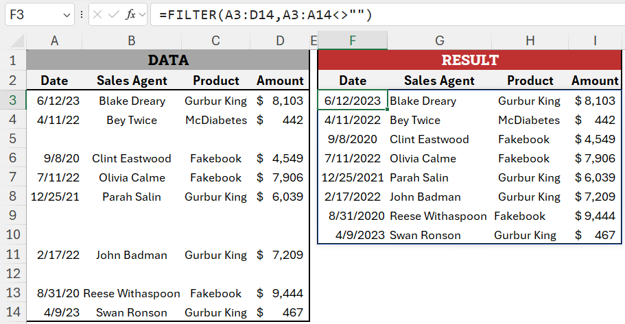
Basically, we checked the first column for blank or empty cells with A3:A14<>”” criteria argument and it helped us remove empty rows.
However, situation changes if the first column is not empty.
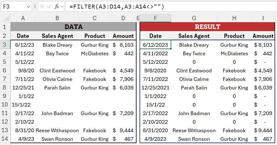
In this case, we cannot rely solely on one column to identify blank rows in the data as we need to check each column individually for empty cells.
This asks for multiple AND criteria expression i.e. criteria for each column will be joined using asterisk (*) operator. The formula is:
=FILTER(A3:D14,(A3:A14<>"")*(B3:B14<>"")*(C3:C14<>"")*(D3:D14<>""))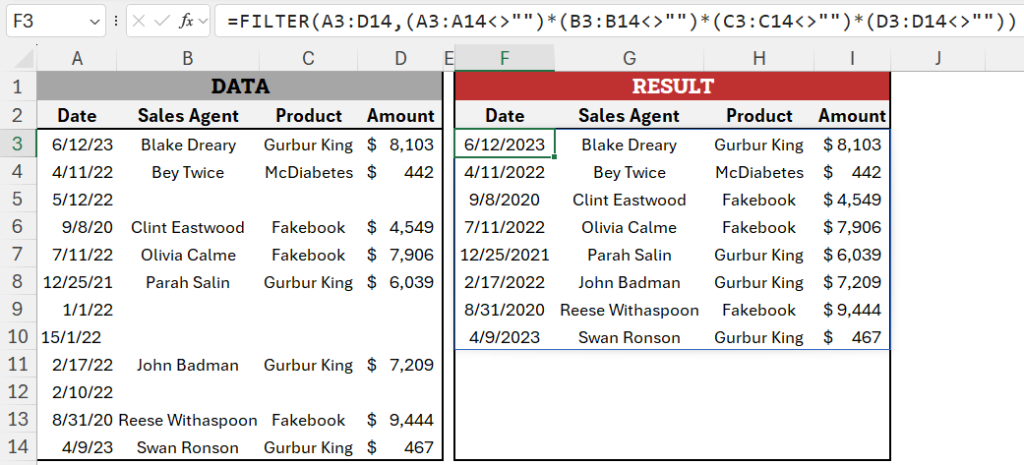
FILTER + BYROW Function To Remove Blank Rows
Though above approach works perfectly for us, but it can quickly become impractical if we have large number of columns. In that case, selecting each column and checking them for blanks is unworkable.
One could have thought of selecting the entire data instead of selecting each column individually, but with array of arrays limitation, Excel cannot process such criteria just yet and throws a #VALUE! error.
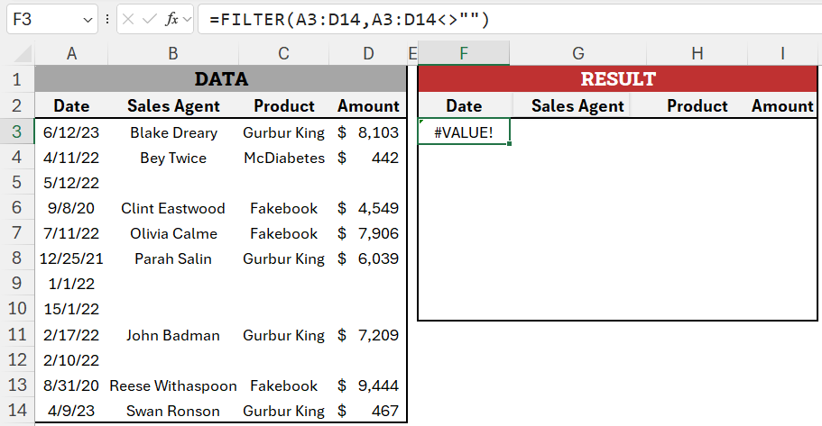
For now, FILTER function can process array of values as criteria rule i.e. it expects a single value for each line item or simply stating one-dimensional 1D array.
Just like we saw in case of A3:A14<>””. As we are checking a single column, the output is a single value each line and FILTER function was able to process it.
In case of A3:D14 we get array of TRUEs and FALSEs for each line item or in other words a two-dimensional 2D array. Here is the formula:
=A3:D14<>""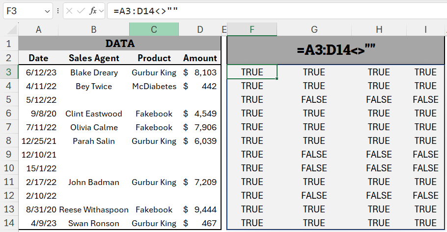
As stated earlier, FILTER function can take one value each line, we need to find a way to “summarize” each line to a single value in such a way that it still help us identify rows with complete records i.e. rows without blanks.
A row is complete or without blanks if all values in the row return TRUE. Even if one value is FALSE this means blank cells and must be excluded. This is exactly what AND criteria is.
Running each line with AND function, we can identify the rows that are complete or without blanks as only such rows will return TRUE. Any row with blanks will return FALSE.
Use this formula and drag the fill handle down to process each row:
=AND(F3:I3)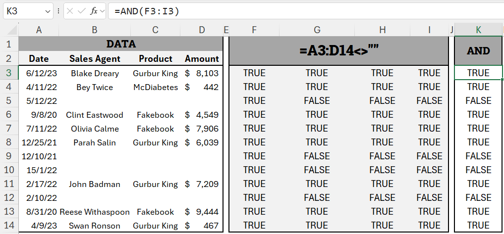
Here we can take help of BYROW function that runs through each row automatically for us and save us from manually writing and dragging the formula down to fill the range:
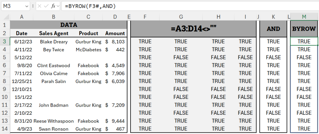
Notice F3# that formula recognized a dynamic array output and selected such range using a hash operator within the formula. We can replace it with the actual formula in cell F3 to save ourselves from helper array. And the formula will become:
=BYROW(A3:D14<>"",AND)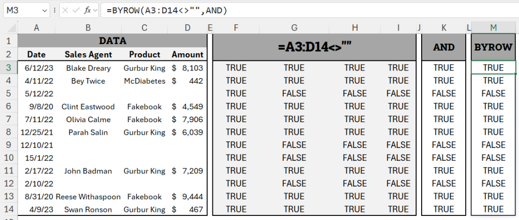
This is where we can combine FILTER function with BYROW function to check each row has complete set of records and remove it if its not.
In other words, using we can remove both completely and partially blank rows in Excel using formula with FILTER and BYROW functions:
=FILTER(A3:D14,BYROW(A3:D14<>"",AND))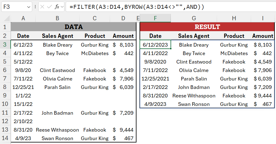
Remove Completely Blank Rows Only
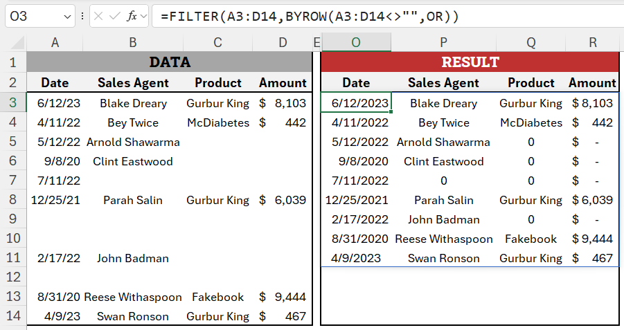
If we like to delete only such rows that are completely empty leaving the partially complete rows in results, we can use the same FILTER + BYROW with a small change.
Instead of AND criteria, we need to go with OR criteria.
Remember:
- AND criteria returns TRUE only if all the conditions return TRUE and will output FALSE even if one condition is FALSE. Using AND criteria in this case will eliminate both completely empty and partially empty rows.
- OR criteria returns TRUE even if one condition out of all is TRUE and will output FALSE if all the conditions return FALSE. Using OR criteria in this case will eliminate only completely empty rows.
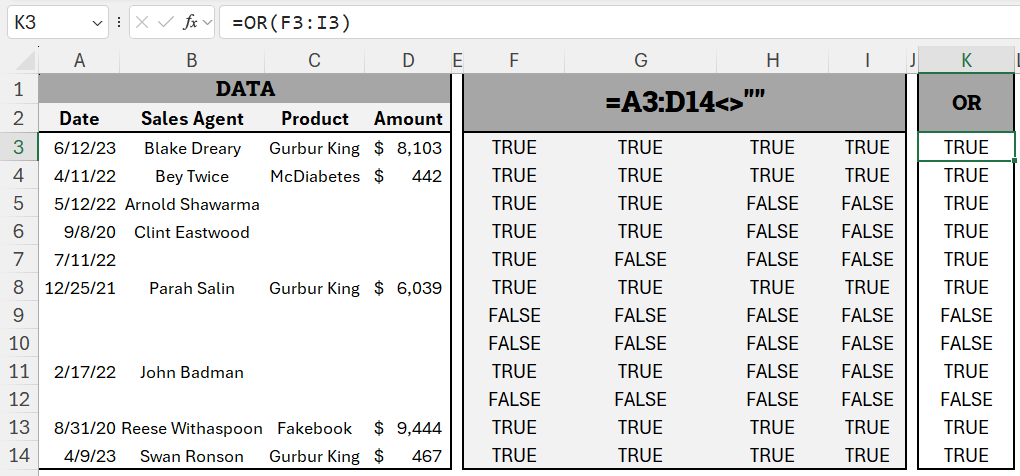
Again, instead of writing the OR formula manually and dragging the fill handle down, we can we can use the following BYROW formula:
=BYROW(A3:D14<>"",OR)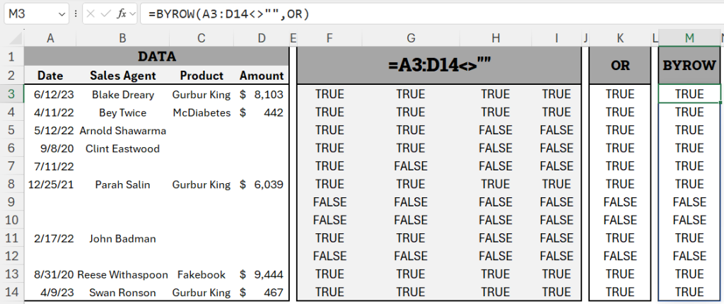
Taking the BYROW formula as include argument for FILTER function, we get a formula that removes completely blank rows leaving the partially blank rows intact:
=FILTER(A3:D14,BYROW(A3:D14<>"",OR))